Load Case vs Load Step
It might happen that new starters in Structural Analysis based on Finite Element Models tend to get confused by what is a Load Case with what is a Load Step.
The Load Case is used in linear static analyses and it is composed by a set of forces, moments, pressures, temperature distributions and boundary conditions. An analysis can have several Load Cases and for each of them a set of results is calculated by the Finite Element code in use, i.e. each Load Case is independent from all the others.
The Load Step, on the other side, is used in non-linear analyses (large deflections, contacts, material plasticity) and it is still defined by assigning forces, moments, pressures, temperature distributions and boundary conditions, but each Load Step (if more that one is foreseen) is dependent from the previous one, so that the sequence of Load Steps defines a loading history; as an example, if we had bolt pretension in our model, the preload has to be applied at the first Load Step before we can apply the external forces. Inverting the sequence will lead to wrong results, whereas in a situation where we have a linear analysis and two Load Cases the application order is not affecting the results.
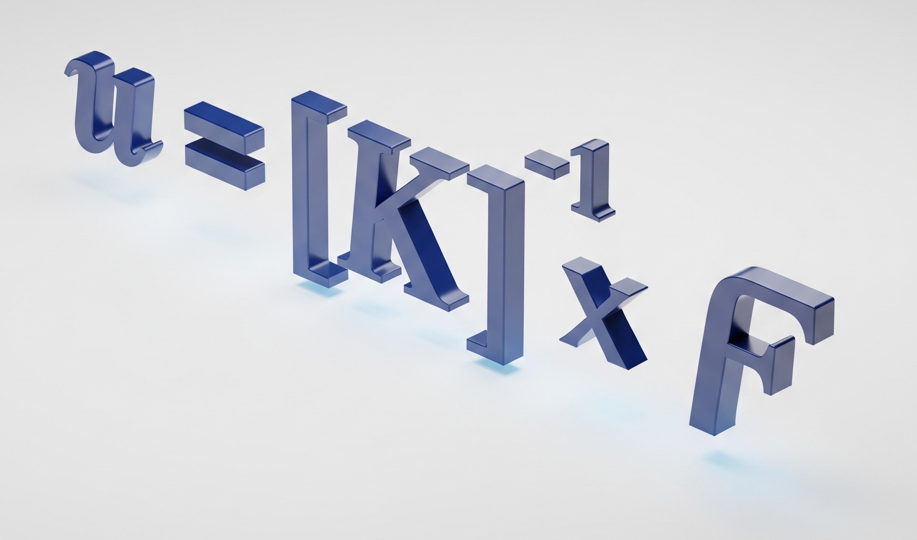
This can be explained by the fact that in linear analysis the stiffness matrix is not a function of the applied loads, whereas for a non-linear analysis the stiffness matrix is dependent on how the structure deforms under the applied loads. It follows that a linear analysis can be “quickly” solved for a huge number of Load Cases with just a unique “inversion” of the stiffness matrix. In fact, as explained in Appendix B of the book “Computational Structural Engineering“, the stiffness matrix is defined by the geometry and the material(s) of the structure to be analysed and eventually by the constraints applied to it; therefore, once the stiffness matrix [K] is “inverted”, to get the solution (that is represented by the displacements vector u) for each Load Case it is sufficient to perform the matrix product [K]‾¹ x F, being F the load vector containing forces, moments, pressures.

Attention must be paid on this point in relation to the Finite Element solver in use; sometimes this aspect is not clear and a misuse of the pre-processor commands can lead to uselessly complications, i.e. using Load Steps instead of Load Cases, will force the code to invert the (same) stiffness matrix for each load condition.
We conclude by highlighting that, on the other side, a non- linear analysis might require the stiffness matrix to be inverted for every load increment (that is a fraction of the applied loads) within a single Load Step and strategies are put in place by the code developers to minimize those inversions without jeopardizing the quality of the results.
A final note
Here we talked about the “inversion” of the stiffness matrix as a pure concept: in reality FE codes do not actually invert the matrix, because it is computationally inefficient; othher numerical techniques are instead put in place to minimize the number of operations required to “factorize” [K].
A similar speech, clearly, applies to the matrix product u = [K]‾¹ x F.
