15.08.2026 – Nodal Mass Distribution and Kinetic Energy Evaluation in Abaqus/Explicit: Element Centroids vs. Nodal Lumped Mass Formulations
Executive Summary
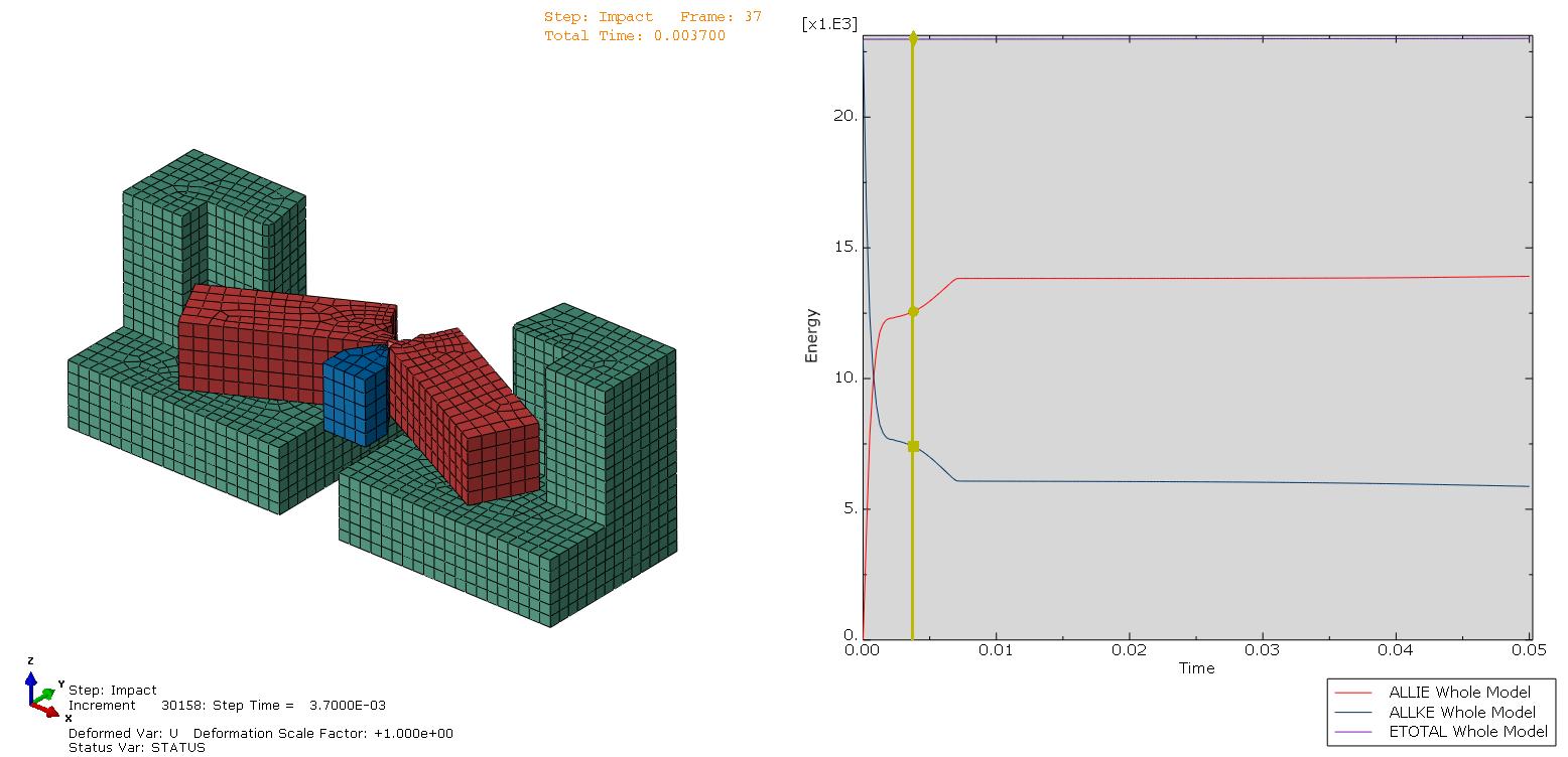
In high-velocity explicit dynamic simulations—such as containment tests, rotor burst analyses, and Charpy impact tests—engineers often observe discrepancies between the global kinetic energy reported by Abaqus (ALLKE) and custom kinetic energy calculations executed via post-processing Python scripts. This technical paper clarifies the theoretical and algorithmic root causes of these discrepancies.
Specifically, we demonstrate why element-centroid velocity averaging underestimates kinetic energy compared to the nodal lumped mass formulation, mathematically analyze the impact of high rotational velocity (König’s Theorem), and address the handling of mass conservation in eroded elements (STATUS = 0). Finally, we present an authoritative methodology for extracting accurate fragment kinetic energies using the Abaqus Python ODB API.
1. Introduction & Problem Statement
In explicit time integration schemes (such as the central difference method implemented in Abaqus/Explicit), tracking energy quantities is crucial for validating energy balance and assessing structural containment capabilities.
A common post-processing requirement involves evaluating the remaining kinetic energy of debris or uncontained high-speed fragments (e.g., turbine blades or compressor impellers breaching a casing). Engineers frequently write custom Python post-processing scripts to sum the kinetic energy of selected element sets (Ek, elem):
However, when comparing ∑ Ek, elem against Abaqus’s internal whole-model kinetic energy history output (ALLKE), two major discrepancies arise:
- Underestimation of Kinetic Energy: Ek, elem is systematically lower than
ALLKE, even prior to material failure. - Severe Divergence During Fracture: Upon element deletion (
STATUS = 0), Ek, elem drops sharply toward zero, whereasALLKEremains continuous and physically conserved.
2. Theoretical Foundations
2.1 The Nodal Lumped Mass Matrix (M) Formulation
Abaqus/Explicit uses a diagonal (lumped) mass matrix M computed at the beginning of the step (t = 0). The global kinetic energy Tglobal computed internally by the solver for N total nodes is expressed as:
where mn, i is the lumped mass assigned to node i, and vx, i, vy, i, vz, i are the translational velocity components of node i.
For standard linear isoparametric continuum elements (such as 8-node hexes C3D8R or 4-node tetrahedra C3D4), the total element mass me = ∫ ρ dV0 is distributed uniformly among its constituent nodes:
Because the lumped mass matrix is uncoupled, rotational inertia at the element level is represented entirely by the translational velocity gradients across the element’s nodes.
2.2 Rotational Energy and König’s Theorem
When an element undergoes rigid-body rotation or spatial deformation, evaluating kinetic energy using only the centroidal translational velocity vcentroid neglects higher-order kinematic terms.
According to König’s Theorem, the total kinetic energy T of a deformable discrete system of particles (or element nodes) with mass M = ∑ mi is decomposed into:
where vCM is the center-of-mass velocity of the element.
- Centroid-Based Method: Evaluates only Ttranslation = ½ M ‖vCM‖2.
- Nodal Summation Method: Captures both Ttranslation and Trotation/relative.
2.3 Mass Conservation and Element Erosion (STATUS = 0)
In Abaqus/Explicit, when an element satisfies a damage/fracture criterion (e.g., Johnson-Cook or ductile failure), the element is eroded (STATUS = 0).
- Element State: The element’s stress tensor and internal stiffness are zeroed, and its volume variable
EVOLbecomes zero or undefined in subsequent output frames. - Nodal State: The mass allocated to the element’s nodes is NOT destroyed. The nodal lumped masses mn, i calculated at t = 0 remain frozen throughout the analysis. Free unattached nodes (“orphan nodes”) continue to fly through space according to Newton’s First Law.
ALLKECalculation: Abaqus computesALLKEusing the complete nodal vector. Therefore,ALLKEconserves mass and kinetic energy across element erosion events (eroded mass kinetics).
3. Recommended Scripting Methodology (Python ODB API)
To accurately compute kinetic energy for post-processing—matching Abaqus ALLKE or isolating specific high-velocity fragment sets—the post-processing algorithm must operate on nodal lumped masses frozen at t = 0.
Algorithmic Workflow:
- Initialization Step (t = 0, Frame 0):
- Extract initial element volume V0, e (
EVOL) and initial density ρ0, e (DENSITY). - Compute initial element mass: me = ρ0, e · V0, e · EMSFe (accounting for Mass Scaling if applied).
- Distribute me equally among element connectivity nodes to assemble a static nodal mass dictionary:
node_mass_map[nodeLabel].
- Extract initial element volume V0, e (
- Evaluation Step (Time t, Frame k):
- Retrieve nodal velocity vectors vi = (vx, i, vy, i, vz, i) from field output
V. - For the target region or spatial bounding domain (e.g., nodes located outside the casing geometry), evaluate:
Ek, nodal = ∑ ½ ·
node_mass_map[i] · ( vx, i2 + vy, i2 + vz, i2 )
- Retrieve nodal velocity vectors vi = (vx, i, vy, i, vz, i) from field output
4. Key Takeaways and Best Practices
| Aspect | Element-Centroid Method | Nodal Lumped Mass Method (Recommended) |
|---|---|---|
| Formulation | Sum of element mass × centroid velocity squared | Sum of nodal lumped mass × nodal velocity squared |
| Rotational Energy | Ignored (Translational mode only) | Fully captured (Translational + Rotational) |
Eroded Elements (STATUS=0) |
Lost (yields zero volume/mass) | Preserved via frozen t = 0 nodal mass matrix |
Agreement with ALLKE |
Poor (underestimates energy) | Exact / Complete alignment |
| Primary Use Case | Quick spatial visualizations | Accurate fragment energy & containment verification |
5. Conclusion
Evaluating kinetic energy in explicit dynamics requires strict alignment with the numerical formulation of the solver. Because Abaqus/Explicit integrates equations of motion at the node level via a diagonal lumped mass matrix, post-processing calculations of kinetic energy must likewise be evaluated at the nodes.
By freezing nodal lumped masses at t = 0 and applying current nodal velocities, analytical engineers can accurately capture both translational and rotational kinetic energy—even in the presence of severe element erosion and high-velocity fragmentation.
