Fatigue Assessment in Structural Engineering: From Core Methodologies to the Dimensional Size Factor
Executive Summary
Fatigue failure remains the leading cause of structural breakdown in industrial machinery, automotive structures, and aerospace components. Performing a rigorous Fatigue Assessment in Structural Engineering requires much more than extracting maximum Von Mises stress values from a static Finite Element Analysis (FEA) model and comparing them to standard material handbooks. Engineers must bridge the gap between idealized laboratory test specimens and real-world industrial components. This white paper clarifies core fatigue methodologies—such as stress-life approaches, multiaxial fatigue criteria, and damage accumulation—while detailing the often-overlooked role of the dimensional size factor in modifying material endurance limits.
1. Clarifying Fatigue Assessment Methodologies in FEA
A frequent misconception in structural design is treating fatigue analysis as a simple derivative of static strength calculations. In reality, fatigue damage is a localized, progressive mechanism governed by cyclic stress ranges, mean stress shifts, material micro-defects, and geometric stress concentrations.
Stress-Life (S-N) vs. Strain-Life (e-N) Approaches
Depending on the operating regime, structural engineers must adopt the appropriate fatigue formulation:
- High Cycle Fatigue (HCF / Stress-Life): Applicable when operational stresses remain well within the elastic range (typically N > 105 cycles). It relies on standard Wöhler (S-N) curves and stress ranges (Δσ).
- Low Cycle Fatigue (LCF / Strain-Life): Required when localized yielding occurs at notch roots or severe stress concentrations (typically N < 104 cycles). It uses the Coffin-Manson relation to account for plastic strain amplitudes.
Nominal vs. Local Stress Approaches
When processing FEA results, comparing raw FEA nodal stresses directly to smooth speciment fatigue limits can yield severely erroneous fatigue life estimates:
- Nominal Stress Method: Evaluates global cross-sectional stresses against standardized S-N curves that already incorporate geometric fatigue notch factors (Kf).
- Hot-Spot / Local Stress Method: Uses localized structural stresses at weld toes or notch roots, separating membrane and bending stress components to account for local strain magnification.
Multiaxial Fatigue Considerations: Uniaxial stress states rarely exist in real operating structures. When principal stress directions rotate during cyclic loading, classical scalar criteria fail. Advanced multiaxial criteria (such as the critical plane approache) must be implemented in FEA post-processing to accurately predict fatigue initiation under non-proportional loading.
2. Variable Amplitude Loading and Cumulative Damage
Real-world operational load histories are rarely constant-amplitude sine waves. Complex duty cycles generate irregular load-time histories that must be translated into discrete stress cycles.
The industry standard procedure involves two primary steps:
2. Palmgren-Miner Linear Damage Rule: Calculates cumulative fatigue damage D:
D = ∑ (ni / Ni) ≤ Dcritical
Where ni is the applied number of cycles at stress level i, and Ni is the allowable number of cycles to failure at that same level on the modified S-N curve. While Dcritical is theoretically equal to 1.0, it is recommended to lower the design threshold (e.g., 0.3 to 0.5) to account for sequence effects and material scatter.

3. The Dimensional Factor in Fatigue Analysis (Size Effect)
Even when stress concentrations and surface roughness are properly accounted for, large industrial components systematically exhibit lower fatigue endurance limits than small laboratory specimens. This phenomenon is known as the size effect or dimensional factor (b3 or Csize).
Standard fatigue limits published in material databases are generally derived from standard polished rotating-bending test specimens with a typical diameter of d0 ≈ 7.5 mm to 10 mm. When scaling up to real component dimensions (e.g., shafts of 100 mm or structural beams of 500 mm), the fatigue endurance limit drops significantly.
Why Does Component Size Reduce Fatigue Strength?
The dimensional size effect is driven by two distinct physical mechanisms:
- Statistical Effect (Defect Distribution): Fatigue crack initiation originates at microstructural flaws, non-metallic inclusions, or surface defects. A larger structural volume (or surface area) contains a statistically higher probability of harboring a critical flaw, so that larger components fail at lower mean stress levels.
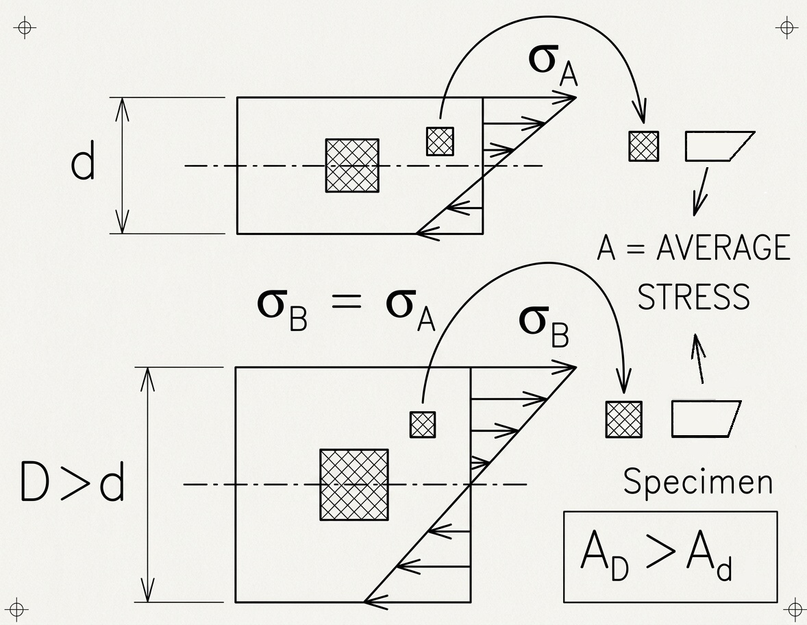
- Geometrical / Stress Gradient Effect: Under bending or torsional loading, the stress distribution is non-uniform. In a small diameter pin, the stress drops rapidly away from the surface (steep stress gradient). In a large shaft, the stress gradient is much shallower, resulting in a higher mean stress acting on the “grain” of material, as shown in the figure here below.
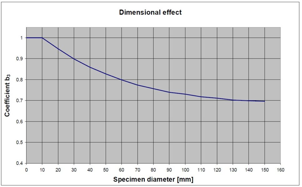
Quantifying the Size Factor b3: Under pure axial tension, the stress gradient effect vanishes, leaving only the statistical defect volume effect. Under bending and torsion, however, the size factor b3 decreases sharply as diameter increases, as shown in the graph below.
On the basis of this experimental evidence, nowadays more and more frequently axial tests are used instead of rotating bending, so that there is no stress gradient; the machines required are somewhat more complex and these tests are, therefore, more expensive.
Several comparisons between the rotating bending test and the axial test on the same material have shown a relationship between the two fatigue limits obtained:
“Faa” being the axial alternating fatigue limit and “Fab” the bending alternating fatigue limit. From here it can be seen that the axial tests give more conservative values.
4. Integrating Size Factors and Stress Gradients in FEA Workflows
Modern FEA-based fatigue post-processors go beyond simple empirical empirical diameter-lookup tables. By leveraging full 3D stress fields, advanced solvers evaluate local stress gradients directly from the finite element mesh:
- Stress Gradient Extraction: The post-processor calculates the relative stress gradient χ = (1/σmax) · (dσ/dx) perpendicular to the critical surface point.
- Highly Stressed Volume (HSV): The solver integrates the surface area or volume exposed to stress levels close to the peak value, automatically adjusting the local fatigue limit based on exact component geometry rather than simple equivalent cylinder assumptions.
- Mesh Dependence Management: High stress gradients require localized mesh refinement. Using gradient-based fatigue algorithms helps mitigate artificial mesh sensitivity at sharp re-entrant corners.
5. Conclusion
Conducting an accurate Fatigue Assessment in Structural Engineering requires a holistic approach that bridges theoretical mechanics with practical FEA post-processing. Ignoring the dimensional size factor or relying solely on uncorrected elastic FEA stress peaks will result in either dangerously unconservative fatigue life predictions or over-engineered, excessively heavy structures.
By properly combining stress-life methodologies, rainflow cycle counting, multiaxial criteria, and gradient-based size effect corrections, engineers can unlock reliable fatigue predictions and optimize component mass with confidence.
In Chapters 10 of my book, Computational Structural Engineering, I detail the complete mathematical framework for multiaxial fatigue, showing how to handle and use FEA results into practical methods, up to implementing stress gradient size corrections inside industrial FEA workflows.
