The SAFE Interference Diagram for the Design of a Compressor Impeller

Document Type: Technical Article / Turbomachinery Integrity

Domain: Centrifugal Compressors, Structural Dynamics, Resonance Evaluation, Pre-Stressed Modal Analysis

Keywords: SAFE Interference Diagram, Impeller, Modal Analysis, Resonance, Nodal Diameter, Harmonic Index, Abaqus, CG CAE

Abstract

Open impellers serve as critical rotating components within centrifugal compressor systems, making their mechanical integrity central to operational reliability. Structural evaluation typically spans both static assessment under steady operating loads and pre-stressed modal analysis to map harmonic response characteristics and avoid dynamic resonance risks. The Singh’s Advanced Frequency Evaluation (SAFE) Interference Diagram provides a comprehensive analytical framework by unifying natural vibration frequencies, disk mode shapes, rotational speed limits, and excitation frequencies into a single diagnostic chart. This paper presents the core methodology of the SAFE Diagram alongside representative pre-stressed cyclic modal results computed in Abaqus.

1. Bladed Impeller Vibration and Dynamic Resonance

Resonant vibration driven by cyclical flow pressure distortions represents a primary failure mechanism in open bladed impellers. As the bladed disk rotates past static upstream inlet vanes or downstream diffuser passages, individual blades encounter pressure fluctuations occurring at discrete multiples of the rotational speed. Resonance occurs when two distinct conditions coincide simultaneously:

The frequency of the periodic flow perturbation matches an undamped natural frequency of the rotating assembly.
The spatial force profile aligns with the structural mode shape associated with that natural frequency.

Exploiting the rotational symmetry of axisymmetric structures allows the global dynamic behavior to be evaluated using a single repetitive sector containing one blade and its associated disk segment. Two fundamental descriptors define this spatial response:

Nodal Diameters and Nodal Circles (d)

Nodal lines identify stationary locations across the disk surface where out-of-plane axial displacement remains zero during vibration. Radial stationary lines correspond to nodal diameters, which naturally occur as orthogonal mode pairs at a given natural frequency. Concentric stationary rings indicate nodal circles (umbrella modes). Radial and circumferential wave patterns combine to produce increasingly intricate mode shapes at higher frequencies.

Harmonic Index (HI)

The Harmonic Index characterizes phase relationships between adjacent repeating sectors in an N-sector symmetric structure. Relative blade displacement fluctuates between in-phase and out-of-phase motion. The maximum achievable Harmonic Index depends directly on sector count:

HI = (N − 1) / 2 (for odd N)

HI = N / 2 (for even N)

The total number of nodal diameters d correlates with the Harmonic Index and sector count N through integer multipliers m (where m = 0, 1, 2, 3, …):

d = m · N ± HI

m	Harmonic Index (HI)
m	0	1	2	3	4
0	d = 0	d = 1	d = 2	d = 3	d = 4
1	d = 9	d = 8	d = 7	d = 6	d = 5

Table 1: Relation between Nodal Diameters (d) and Harmonic Index (HI) for a no-bladed disk with 9 sectors.

Mathematical Formulations for Harmonic Forcing and Energy Work

For an unforced, undamped Single Degree of Freedom (SDOF) structural system, governing motion follows:

M · x”(t) + K · x(t) = 0

where mass M and stiffness K remain constant, yielding the harmonic displacement response:

x(t) = A · cos(ω_nt + φ)

External forcing F(t) expands into a Fourier series dependent on rotational speed (RPM) and the number of stationary flow obstructions P:

ω_P = ( Speed_RPM · P ) / 60 [Hz]

F_P(θ, t) = F_P · sin(ω_Pt + Pθ)

For a vibration mode shape defined by d nodal diameters and natural frequency ω_d:

x_d(θ, t) = −A_d · cos(ω_dt + dθ)

Energy transfer work W per vibration cycle indicates whether forcing energy fuels sustained resonance:

W = π · Speed_RPM · F_P · A_d (when d = P and ω_d = ω_P)

W = 0 (when d ≠ P or ω_d ≠ ω_P)

Consequently, excitation harmonics P exceeding the maximum structural HI can still induce resonance, provided the nodal diameter spatial match (P = d) and frequency equality conditions are met.

2. The SAFE Interference Diagram

The Singh’s Advanced Frequency Evaluation (SAFE) Interference Diagram projects natural frequencies, Harmonic Index values, nodal patterns, and operational speed ranges onto a unified diagnostic plane.

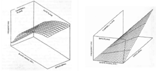
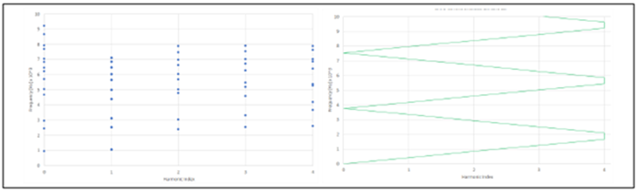
3D Presentation of Modal Impeller Parameters and Force Excitation

Figure 1: 3D presentation of modal impeller parameters (right: vibrating impeller parameters; left: force excitation).

By superimposing structural parameters alongside operational speed curves within a 3D coordinate frame, two analytical projections emerge: the Campbell diagram (frequency vs. speed) and the SAFE diagram (frequency vs. Harmonic Index). The SAFE chart displays natural mode frequencies plotted against Harmonic Index alongside folded speed excitation lines reflecting spatial aliasing. Intersections between structural frequency points and speed lines highlight potential operational resonance points.

SAFE Interference Diagram - Frequency vs HI and Speed Lines

Figure 2: SAFE Interference Diagram (left: frequencies at HI; right: rotational speed).

3. Pre-Stressed Modal Cyclic Analysis in Abaqus

To demonstrate this methodology, an open centrifugal impeller featuring 17 repeating sectors (N = 17) was modeled in Abaqus. Centrifugal loading from maximum operational speed was first applied within a static analysis step to establish the pre-stressed state. A pre-stressed modal analysis was subsequently performed on a single sector utilizing Abaqus cyclic symmetry options to solve for all Harmonic Index modes.

Cyclic Symmetry Advantages: Modeling a single sector with cyclic symmetry boundary conditions drastically reduces computational costs while accurately capturing full 360-degree bladed disk interaction modes across all Harmonic Index orders.

HI	Frequency [Hz] / Mode Shape
HI	Mode 1	Mode 2
0	909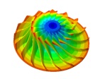	1440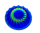
1	1367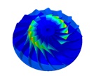	1734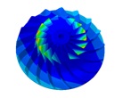
2	1385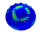	1899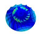
3	1425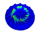	2040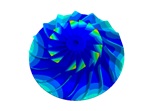
4	1464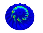	2232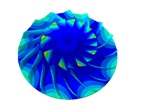
5	1492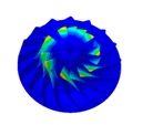	2485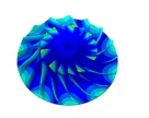
6	1509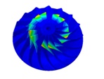	2764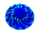
7	1519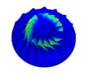	2963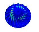
8	1523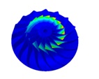	3027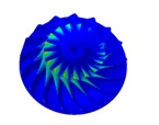

Table 2: Calculated natural frequencies and associated mode shapes for each Harmonic Index (HI 0 through 8) in Abaqus.

4. Evaluating SAFE Interference Results and Design Margins

Plotting the computed modal frequencies against the rotational speed forcing lines (incorporating a ±10% operational safety margin band) yields the complete SAFE Interference Diagram for the 17-sector impeller assembly.

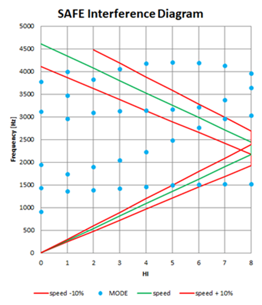
SAFE Interference Diagram with Speed Line and Margin Bands

Figure 3: SAFE Interference Diagram displaying computed natural frequency points alongside operational speed line and ±10% frequency margin bands.

In the analyzed operating range, direct intersections between primary speed lines and natural frequencies are avoided. However, evaluating potential vane passing frequencies from stationary components reveals that choosing 5, 6, 10, 11, or 12 stationary vanes would place excitation harmonics inside the 10% safety margin. This chart enables engineers to select stationary vane counts (such as inlet guide vanes or diffuser vanes) that maintain adequate frequency clearance.

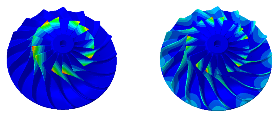
When potential margin conflicts occur, evaluating mode shape characteristics helps determine whether excitation acts primarily at the Leading Edge (LE) or Trailing Edge (TE) of the blades. Mode shapes focusing deformation near the LE indicate susceptibility to upstream disturbance, whereas TE-dominated modes react primarily to downstream diffuser effects.

Impeller Mode Shapes at 1509 Hz and 2764 Hz

Figure 4: Mode shape contours at 1509 Hz (d = 6, LE deformation dominant) and 2764 Hz (d = 11, combined LE/TE deformation).

5. Conclusion

The SAFE Interference Diagram provides a reliable methodology for evaluating dynamic vibration risks in open compressor impellers. By consolidating natural frequencies, spatial mode shapes, rotational speeds, and forcing harmonics into a single diagnostic framework, it allows design teams to optimize stationary vane counts, verify frequency safety margins, and target forced response analyses effectively.

References

[1] Wang Q., Bartos J., Houston R.: “Methodology of open bladed impeller resonance identification”, Proceedings of 28th Turbomachinery Symposium, 1999.
[2] Singh M.: “SAFE Diagram – A Dresser-Rand Evaluation Tool For Packeted Bladed Disc Assembly”, Dresser-Rand TP025.
[3] Singh M. P., Vargo J. J., Schiffer D. M., Dello J. D.: “SAFE Diagram – A design and reliability tool for turbine blading”, Proceedings of 17th Turbomachinery Symposium, 1988.
[4] Singh M., Thakur B. K., Sullivan W. E., Donald G.: “Resonance Identification for Impellers”, Proceedings of 32nd Turbomachinery Symposium, 2003.
[5] Singh M., Drosjack M.: “Emerging advanced technologies to assess reliability of industrial steam turbine blade design”, Proceedings of 37th Turbomachinery Symposium, 2008.
[6] Singh M.: “History of evolution, progress and application of SAFE diagram for tuned and mistuned system”, Proceedings of 42nd Turbomachinery Symposium, 2013.
[7] Dello J.: “Frequency evaluation of a steam turbine bladed disk”, Turbomachinery International, 1987.
[8] Hassan M.: “Vibratory Analysis of Turbomachinery Blades”, Rensselaer Polytechnic Institute, Hartford, Connecticut, 2008.
[9] Abaqus Documentation, Dassault Systèmes, 2018.